Uncertainty Principle
Pin down exactly where a particle is and you lose all grip on how fast it's going, and the reverse. It isn't clumsy instruments: a wave narrow in space is, unavoidably, broad in momentum. The trade has an exact floor, ℏ/2.
 Open the interactive ▸
 What you're looking at
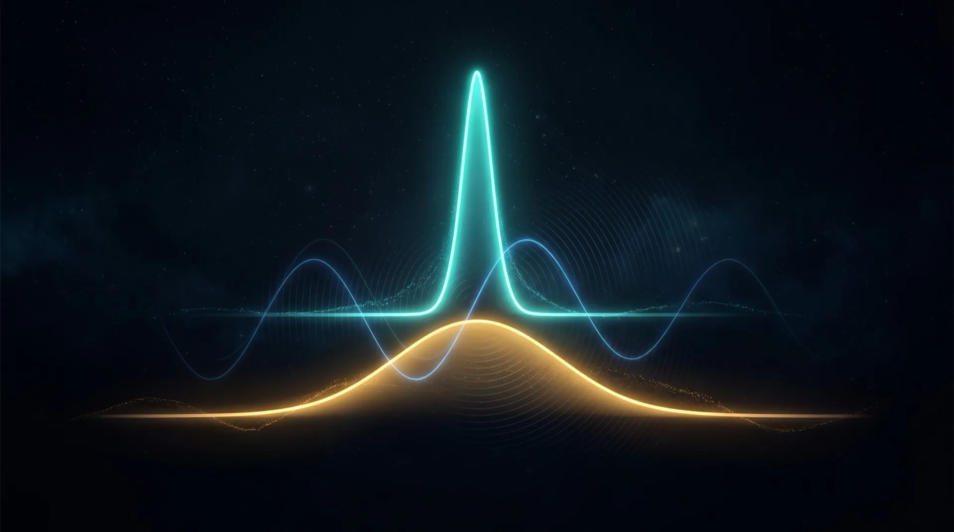
Two pictures of one quantum state. The top curve is |ψ(x)|², the probability of finding the particle at each position. The bottom curve is |φ(p)|², the probability of each momentum. They are not two separate facts; the bottom is the Fourier transform of the top. They're the same wave, written in two languages.
Drag the position spread Δx. As you squeeze the top curve narrow, localising where the particle is, the bottom curve fans out wide: its momentum becomes uncertain. Let the position spread back out and the momentum sharpens. You physically cannot pull both narrow at once. The meter tracks the product Δx·Δp, and it never drops below ℏ/2.
Switch the state: a Gaussian sits exactly on that floor (the best trade nature allows). A two-bump superposition spreads its momentum into interference fringes and floats well above the floor. A flat-top packet's hard shoulders inject extra momentum. Turn on the carrier wave to see the ripples whose wavelength is the momentum, or switch to real scale to watch what confining an electron costs in speed.
Why it's here
This is the fourth and final quantum piece, the keystone of the set. The Double-Slit showed a particle as a wave; the Bell test showed two waves entangled; Tunnelling showed a wave leaking through a wall. Uncertainty names the price of being a wave at all: a wave that is sharp here must be built from many wavelengths, and wavelength is momentum (de Broglie, p = h/λ). So sharp position means blurred momentum, not as a measurement accident, but as a fact of Fourier analysis that was true before quantum mechanics, in every pulse of sound and light.
It's also the antidote to the most common misunderstanding in all of physics. The pop version, "you can't measure something without disturbing it," is Heisenberg's 1927 microscope heuristic, and it's not the principle. The principle, made rigorous by Kennard the same year, is about preparation: no quantum state, however gently you treat it, can have both a definite position and a definite momentum. Looking isn't the problem. Being a wave is.
How it works
For any quantum state, the standard deviations of position and momentum obey Δx · Δp ≥ ℏ/2 (Kennard 1927; generalised by Robertson 1929 to any pair of incompatible observables). The bound is saturated, equality, only by a Gaussian wave packet. That is why the Gaussian state reads exactly 0.500 ℏ here while every other shape reads more.
The reason is the Fourier transform. Position and momentum amplitudes are Fourier conjugates: ψ(x) and φ(p) = FT[ψ]. A basic theorem of Fourier analysis says a function and its transform can't both be arbitrarily narrow, squeeze one, the other spreads, and the product of their widths has a hard minimum. The Gaussian is the unique function that is its own Fourier transform's twin, so it hits that minimum. (The simulation computes Δp the rigorous way, from the wavefunction's slope: ⟨p²⟩ = ∫|dψ/dx|², so the number is exact at any width.)
The everyday consequence is enormous. Δp = ℏ/(2Δx) means confining a particle costs momentum. Pin an electron to within 0.1 nm (an atom's width) and its velocity is uncertain by ~580 km/s, which is why electrons in atoms can't sit still, why atoms have the size they do, and why matter doesn't collapse. The same law in energy–time form, ΔE·Δt ≥ ℏ/2, lets virtual particles borrow energy for a fleeting moment and sets the natural width of every spectral line.
The three states
Three wavefunctions, to feel where the floor is and what rises above it.
- Gaussian (minimum uncertainty). The single shape that saturates the bound: Δx·Δp = ℏ/2 exactly, at any width. Narrow it and the momentum widens in perfect lock-step. This is the gentlest trade the universe permits. Verdict: on the floor.
- Two-bump superposition. The particle's wave is in two places at once, and the two parts interfere in momentum space, carving the distribution into fringes (the same Fourier maths as the double-slit). Its spreads multiply to well above ℏ/2. Verdict: above the floor.
- Flat-top. A boxy packet with steep shoulders. Sharp edges are built from high momenta, so the momentum distribution develops broad tails and the product climbs. Verdict: above the floor.
Accuracy
The honest line between what is exact and what is dialled for display:
| Feature | Tier | What that means |
|---|---|---|
| The bound Δx·Δp ≥ ℏ/2 | T1 Established | Kennard's theorem (1927); Robertson's general form (1929). A proof about standard deviations, not a measurement limit. |
| Gaussian saturates the bound (= ℏ/2) | T1 Established | The Gaussian is the unique minimum-uncertainty state. The simulation reads exactly 0.500 ℏ for it at every width. |
| Position and momentum are a Fourier pair | T1 Established | φ(p) = FT[ψ(x)]; the bottom panel is literally the Fourier transform of the top. The reciprocal spreading is a Fourier theorem. |
| Real consequence (electron confined to Δx → Δv) | T1 Established | Δp = ℏ/(2Δx); for an electron in 0.1 nm, Δv ≈ 580 km/s. Real number, and why atoms have size. |
| Energy–time form ΔE·Δt ≥ ℏ/2 | T1 Established | The same relation for energy and duration: line widths, virtual particles, lifetimes. (Δt is interpreted carefully, not as an observable.) |
| It is about preparation, not measurement disturbance | T2 Theoretical | Heisenberg's 1927 microscope story conflated the two. The modern view (Busch–Lahti–Werner 2013; Ozawa 2003) keeps a separate, refined error–disturbance relation. Still actively discussed. |
| Whether "the particle has a definite x and p we just can't know" | T2 Theoretical | Hidden-variable readings differ from the orthodox "no joint value exists." (See the Bell test next door.) Interpretation. |
| Display units; Δx read as nanometres for the real-scale figure | T3 Stylised | The maths is unit-free (ℏ); the nm/electron mapping is a chosen real-world anchor. |
| The carrier-wave animation; chosen example states | T4 Illustrative | The moving ripples are a visual aid (phase, not |ψ|²); the three states are representatives, not an exhaustive set. |
In one line: the ℏ/2 bound, the Gaussian saturating it, the Fourier-pair relationship and the real electron numbers are exact, established physics; only the display units and the carrier animation are dialled for clarity, and "is it really there but unknowable?" is the part that connects to interpretation, and to Bell.
Sources
- Heisenberg, W. (1927). Über den anschaulichen Inhalt der quantentheoretischen Kinematik und Mechanik. Z. Phys. 43, 172. The original paper, and the microscope heuristic.
- Kennard, E. H. (1927). Zur Quantenmechanik einfacher Bewegungstypen. Z. Phys. 44, 326. The rigorous σ_x σ_p ≥ ℏ/2.
- Weyl, H. (1928). Gruppentheorie und Quantenmechanik. Independent derivation of the bound.
- Robertson, H. P. (1929). The Uncertainty Principle. Phys. Rev. 34, 163. Generalisation to arbitrary observable pairs.
- Bohr, N. (1928). The Quantum Postulate and the Recent Development of Atomic Theory. Nature 121, 580. Complementarity.
- Ozawa, M. (2003). Universally valid reformulation of the Heisenberg uncertainty principle. Phys. Rev. A 67, 042105. Refined error–disturbance relation.
- Busch, P., Lahti, P., & Werner, R. F. (2013). Proof of Heisenberg's Error-Disturbance Relation. Phys. Rev. Lett. 111, 160405. The measurement-vs-preparation clarification.