The Wave Schedule
The most famous graph in the UFO literature is a question: Vallée's Figure 3, the waves of 1947-1962 with the trend removed, captioned "Is this a schedule of reinforcement?" The catalogue behind it was private and the figure cannot be recomputed, so for fifty years the question has been answered by eye. The public record that carries the same waves can be recomputed by anyone, and this bench does, with every load-bearing word on a dial. Turn the threshold to 2σ inside Vallée's window and the famous five-year clock is really there: July 1947, July 1952, November 1957, spaced 60 and 64 months. Press one button to extend the record and the next wave arrives 93 months late. Ask the spectrum: against the shuffled-months null the wave periods shine, which is why every generation sees cycles here; against surrogates that carry the record's own burstiness, nothing longer than a year survives except the seasonal line, eleven times the noise, July 78 to January 30. Ask Skinner's gauge: six waves, five intervals, a CV whose confidence interval covers the clock and the variable schedule at once. The two biggest months in the file are the Washington summer the press ran ahead of, and the month Sputnik 2 rose over Levelland. The bench computes all of it and votes on none of it.
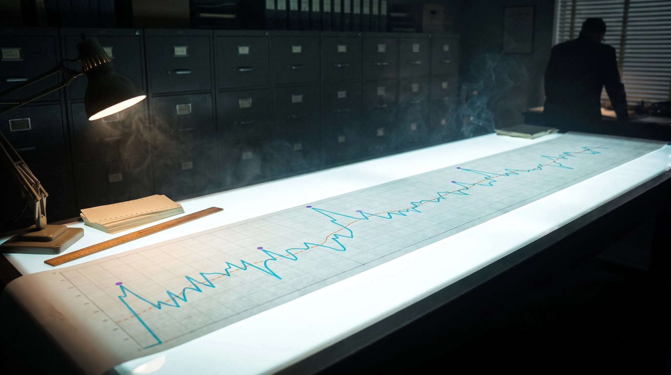 Open the interactive ▸
 What you're looking at
The Index lays out the Blue Book monthly file, 1947-1962 in Vallée's frame or 1947-1969 in full, on a log or linear scale, with the trend drawn as a dashed line whose window is a dial. Below it, the detrended lane Figure 3 lived in: a threshold dial defines what counts as a wave, violet dots mark the detections, and the intervals are labelled in months. The Mars toggle drops the eleven real opposition dates onto the axis.
The Spectrum draws the power of every period at once against a 95% null band you choose: shuffled months, or surrogates carrying the record's own month-to-month memory. The needles never move; only the band does. Markers stand at 12.0 months and at the Mars synodic period of 25.6.
The Schedule is the Skinner machine: the detected waves as a rhythm on one rail, and beneath them fixed-interval, variable-interval and Poisson schedules run at the same rate from fixed seeds. The gauge below computes the interval CV with its bootstrap CI against the three analytic anchors, and answers the caption's question with the only honest answer six waves permit.
The File runs twelve cards: what Figure 3 actually was, where this series comes from, the nine years whose bookkeeping disagrees with itself, Sputnik month, the 1952 summer, Skinner's box, Condon's own health warning, the surge outside the window, the Mars file, and the sentence that closes the loop. Two verdicts hang below at equal size.
Why it's here
The culture wing of this station has just taken in a review of Jacques Vallée's The Invisible College (1975), the book where the control-system hypothesis was first laid down. That review names the book's quantitative heart: Figure 3, a monthly index of UFO activity, 1947-1962, trend removed, captioned "Is this a schedule of reinforcement?", with the whole Skinnerian mechanism standing on it. The review also names it the argument's weakest link: a graph read by eye, built on a private catalogue with unpublished weights, never tested against any null. This instrument was built for that link. Vallée's index cannot be recomputed by anyone; the public record that carries the same waves, the Blue Book monthly file, can be recomputed by everyone. The bench turns the three load-bearing words, wave, period, schedule, into dials, and turns them in front of you.
It is also the station's fourth statistics bench, after INST-37 Project Stargate (what a margin is worth against chance), INST-50 Special Report No. 14 (what a percentage is worth when the denominator moves) and INST-60 The Nuclear Lure (what a correlation is worth against a base rate): this one asks what a rhythm is worth against a null hypothesis. As ever, the answer is not presupposed. At the strict dial inside Vallée's own window the five-year clock is real, 60 and 64 months, and the bench draws it exactly; extend the record to 1969 and the next wave arrives 93 months late and shatters it, and the bench draws that too. Two verdicts hang at equal size in the file, and the dials are yours.
How it works
Everything on the bench is arithmetic on published records: the Condon monthly table, the desk-archive histograms, the programme sheets, and the real Mars dates. A script that ships with the site re-derives every displayed number before the build is allowed to pass, including the places where the record disagrees with itself.
resid = v − CMA_W(v) · wave: resid > θ·σ · CV = sd(Δt)/mean(Δt) · P_k vs 95% of AR(1) surrogates · p_Mars = P_shift(|Δ| ≥ |Δ_obs|)
The definition of a wave is a dial, because the literature never supplied one. A centered moving average removes the trend (window 7-49 months); a wave is a run of residual months above θ·σ merged within a separation dial. Every downstream number inherits these choices visibly. At 1.5σ the record holds six waves; at 2.0σ, three; at 1.0σ, eight.
The null hypothesis is a switch, because it decides the verdict. The same periodogram clears 32, 24 and 21.3 months against shuffled months and clears nothing beyond a year against AR(1) surrogates with the record's own φ = 0.59. The eye is a white-noise instrument; a bursty series manufactures two-year 'cycles' for free. Both bands are drawn from 400 seeded surrogates each.
The schedule question is answered at the sample size the record permits. Skinner's taxonomy separates schedules by interval statistics, and the laboratory needed thousands of trials per animal. The file supplies five intervals; the CV's bootstrap CI spans from near-clockwork to well past the variable schedule. That is not a failure of the bench. It is the finding: the caption's question was unanswerable from its own data in 1975, and it still is.
The Mars test uses circular shifts, not shuffles, because shuffling months would credit the test with destroying the very autocorrelation that produces false hits. The shifts preserve the series' structure and slide the opposition mask around the calendar: 2,000 of them price the observed +20.1 excess at p = 0.13, and dropping the single 1952 coincidence inverts the sign.
What this bench will not do is answer the book's question for you. A trainer permitted to mislead cannot be disproven by any dial, and the bench says so on the card that quotes the sentence. What it can do is separate the checkable from the unfalsifiable: the periodicity is a dial artifact, the unpredictability is what human reporting produces unaided, and the only rhythm the record proves is the year.
The dials that decide what happens
Two windows, two scales, three dials, one null switch. Between them they manufacture and unmake every pattern ever claimed in this series, which is the exhibit.
- The window. 1947-1962 is Vallée's frame, and the five-year clock lives only inside it. 1947-1969 is the out-of-sample test: one button, and the clock meets August 1965.
- The scale. Log compresses the 1952 monster so the early waves exist at all (Vallée's weighting did the same job for his index); linear shows why one month is an eighth of the whole file.
- The trend window. 7 to 49 months. Short windows swallow slow waves into the trend; long ones leave drift in the residual. The default 25 is stated, visible, and movable.
- The threshold and the separation. What counts as a wave, and when two crossings are one wave. The wave count runs from three to eight across honest settings, and every downstream statistic follows it.
- The null switch. White blesses the wave periods; red kills them. The single most consequential control on the bench, and in most published analyses it was never a control at all.
- Mars and labels. The real opposition dates on the axis, and the numbers on or off the charts for reading against screenshots.
The claims, as they stand
Six claims that orbit the wave record, from the book's own caption to the psychosocial null, with where each lands against the arithmetic.
| The waves follow a schedule of reinforcement: periodicity with unpredictability proposed by Jacques Vallée, The Invisible College (1975), Figure 3 | READING | Untestable at the record's sample size, and this bench shows it rather than asserts it: the interval CV's bootstrap CI, [0.08, 0.60], covers the clock and the variable schedule at once. Ferster and Skinner needed thousands of trials to identify a schedule; the file supplies five intervals. The claim's checkable half (periodicity) is a dial artifact; its uncheckable half is guarded by "it MUST mislead us". |
| UFO waves recur on a roughly five-year period proposed by the 1950s literature, from the 1947/1952/1957 spacing | REFUTED | Real at exactly one dial setting inside exactly one window: at 2.0σ, 1947-1962, the three mega-waves sit 60 and 64 months apart. The out-of-sample test kills it: the next wave (August 1965) arrives 93 months after Levelland. No spectral line near 60 months clears any null. |
| The waves follow Mars oppositions proposed by Aimé Michel; tested and abandoned by Vallée himself in the 1960s | REFUTED | Measured here: near-opposition months average 59.1 reports against 39.0, which looks like +51% until the single May 1952 opposition (two months before the biggest wave in history) is removed, at which point the excess inverts to 40.0 vs 43.1. Circular-shift p = 0.13 with it, 0.30 on the full window. Condon's staff printed the same verdict under the same table in 1969. |
| The report series carries a real annual rhythm proposed by every analyst who has touched the file | MEASURED | Measured, and the only rhythm that survives every null: the 12.0-month line at eleven times the white-noise mean, July averaging 78.4 reports to January's 29.8. Summer skies, summer evenings, people outdoors after dark. |
| The waves are self-exciting bursts coupled to attention proposed by the psychosocial reading; Condon's own caption, 1969 | CONTESTED | Consistent with everything measured here: lag-1 memory of 0.59, the Life article preceding the April 1952 jump by days, Sputnik month carrying 361 reports, swamp-gas March 1966 made of coverage of its own explanation. Consistent is not proven: the bench flags that a genuine external schedule would also have to pass through this filter, and could hide under it. |
| The Blue Book monthly record is internally consistent proposed by implicit in every analysis that uses it | REFUTED | Refuted by the record itself: nine of 23 years cannot reconcile their own bookkeeping (1952: months sum 1,503 under a printed 1,501; 1958: 617 under 627; 1966: 1,060 in Condon against 1,112 on the official sheet). Nothing that moves a wave; everything that sets a noise floor under fine-structure claims. |
Try this
- Start on the index at the defaults. Six violet dots, intervals 32, 28, 49, 15, 34. This is the pattern the book heard as a training schedule.
- Turn the threshold to 2.0σ. Three waves: 1947, 1952, 1957, spaced 60 and 64 months. The five-year clock of the 1950s literature, really there, at this dial.
- Now press 1947-1969. The fourth wave lands in August 1965, 93 months late. The clock does not survive its first out-of-sample wave.
- Go to the spectrum on the white null. 32, 24, 21.3 months all clear the band. This is what every eyeball analysis of this file has ever seen.
- Switch to red. One survivor beyond a year: none. The 12.0-month seasonal towers at eleven times the noise. Tap it and read what it means.
- Go to the schedule. Four rails at one rate. Cover the labels and try to tell the record from the Poisson rail. Then tap the gauge and read what five intervals can prove.
- Toggle Mars on the index. The 1952 triangle sits two months left of the 536 spike. Tap it, then read the epoch numbers with and without it.
- End on the file. Read The Exhibit, then The Wobble, then Must Mislead, in that order: what the graph was, what the record is, and why no dial can reach the thesis.
Accuracy
The honest line between what is reported, what is measured, what is modelled on them, and what is a reading:
| Feature | Status | What that means |
|---|---|---|
| The Blue Book monthly record | Reported | The only monthly table of the file ever published: Condon Report, Section V Chapter 2, Table 1 (1950-1967), spliced with the desk-archive histograms for 1947-1949 and the programme's own statistical sheets for 1968-69. 23 years, 12,618 reports by the official yearly totals. Every yearly sum is re-derived against its printed total by the verification script, including the nine years that disagree with themselves. |
| The Mars oppositions | Measured | Eleven real opposition dates, 1948-1969, at a synodic period of 25.6 months. Entered as astronomy, not as claim. |
| Trend and waves | Modelled | A centered moving average with its window on a dial (default 25 months); a wave is a run of detrended months above θ·σ (default 1.5), merged within the separation dial (default 9). At the defaults: six waves, Jul 1947 to Sep 1960, intervals 32, 28, 49, 15, 34 months. At 2.0σ in Vallée's window: exactly the three mega-waves, 60 and 64 months apart. |
| The periodogram and its nulls | Modelled | Plain DFT power of the residual, normalised so white noise averages 1, against the 95th percentile of 400 seeded surrogates: shuffled months (white) or AR(1) series with the record's own lag-1 memory of 0.59 (red). Against white, the wave periods 32, 24 and 21.3 months clear; against red, nothing longer than a year survives except the 12.0-month seasonal at eleven times the noise mean. |
| The schedule gauge | Modelled | The coefficient of variation of the wave intervals, bootstrapped 2,000 times with a fixed seed: CV 0.39, 95% CI [0.08, 0.60] at the defaults. The analytic anchors are 0 for a fixed interval, 0.29 for Skinner's variable interval, 1 for Poisson. The CI covers the first two at once and barely excludes the third: six waves cannot identify a schedule. |
| The Mars epoch test | Modelled | Mean reports within ±2 months of an opposition (59.1) against all other months (39.0), with p = 0.13 from seeded circular shifts that preserve the series' autocorrelation. Drop the single May 1952 opposition and the excess inverts: 40.0 vs 43.1. The periodogram bin nearest the synodic period never clears the red band. |
| Figure 3 itself | Reading | Vallée's exhibit: a private vetted catalogue, weights unpublished, method described in outline. Nothing on this bench is that figure; everything on this bench is its caption, run on the record anyone can check. Whether the rhythm is a schedule is a reading, and the bench declines to make it. |
In one line: the Blue Book monthly record is REPORTED, spliced from its three published sources with every yearly sum re-derived and the nine self-disagreements pinned rather than repaired; the Mars dates are MEASURED astronomy; the trend, the wave set, the periodogram with its two null bands, the CV gauge and the Mars epoch test are MODELLED arithmetic with every model choice on a visible dial and every stochastic figure seeded, re-derived by scripts/wave-schedule-tune.mjs before the build passes; and whether the rhythm is a schedule of reinforcement is a READING the bench declines to make, hanging the schedule and the bursts at exactly equal size. Turn the dials, switch the null, and watch what a rhythm is worth.
Sources
- Edward U. Condon (dir.), "Scientific Study of Unidentified Flying Objects", Section V Chapter 2, Table 1: "Number of UFO Reports Received each Month by Project Blue Book", January 1950 through 1968 as printed (Bantam edition; NCAS and SHG transcriptions cross-checked cell by cell for this bench). The chapter's own caption on the fluctuations, the press-publicity table for 1952 and the Grudge Report No. 6 quotation are from the same chapter.
- Project Blue Book desk records preserved by Rob Mercer: "From the Desks of Project Blue Book: Sightings and Statistics, 1947-1969" (The Black Vault), for the hand-drawn 1947-1949 monthly histograms, the 1966-1969 "Statistical Data" sheets, and the 1949 sheet's three mutually inconsistent totals.
- Air Force fact sheet, "Unidentified Flying Objects and Air Force Project Blue Book": yearly totals 1947-1969 summing 12,618.
- Jacques Vallée, "The Invisible College" (E. P. Dutton, 1975; Anomalist Books 2014), Chapter 9: Figure 3 and its caption, the index-construction sketch, and the reinforcement-schedule argument. Quotations follow the 2014 printing; page references approximate. Reviewed in this site's culture wing.
- C. B. Ferster and B. F. Skinner, "Schedules of Reinforcement" (Appleton-Century-Crofts, 1957), cited in the book as "Patterns of Reinforcement": the schedule taxonomy and the extinction-resistance result the book borrows.
- Jacques Vallée, "Challenge to Science: The UFO Enigma" (with Janine Vallée, Regnery, 1966), for Vallée's own examination and abandonment of the Michel Mars-opposition correlation.
- Mars opposition dates 1948-1969 from the standard astronomical almanac record; synodic period 779.94 days.
- Sputnik 1 (4 October 1957) and Sputnik 2 (3 November 1957) launch dates; Levelland, Texas, 2-3 November 1957; Life, "Have We Visitors From Space?", 7 April 1952; Washington National radar events, 19-20 and 26-27 July 1952; Dexter and Hillsdale, Michigan, 20-21 March 1966, and the 25 March 1966 press conference.